
Learning Objectives
Upon completion of this lesson, BSN students and nursing educators will be able to:
- Distinguish between population distribution, observed sample distribution, and the sampling distribution of a statistic.
- Explain the concept of standard error and calculate it under different conditions.
- Describe the Central Limit Theorem (CLT) and its implications for the distribution of sample means.
- Apply principles of sampling distributions and the CLT to understand and interpret research findings.
Understanding Key Distributions in Statistics
In statistics, particularly in research and evidence-based practice, it is crucial to differentiate between various types of data distributions. This understanding forms the foundation for inferential statistics.
Population Distribution
The population distribution describes the distribution of all possible individual data values for a characteristic of interest within an entire group (the population). For instance, if we consider the blood pressure of all adults in a country, the distribution of these individual blood pressure readings constitutes the population distribution. It has a specific mean (μ) and standard deviation (σ).
Observed Sample Distribution
An observed sample distribution is the distribution of individual data values collected from a single, actual sample drawn from the population. This is the data you directly gather and analyze in a study. For example, if you measure the blood pressure of 100 randomly selected adults, the distribution of these 100 readings is your observed sample distribution. Its characteristics (sample mean, sample standard deviation) are denoted by x̄ and s, respectively.
Sampling Distribution of a Statistic
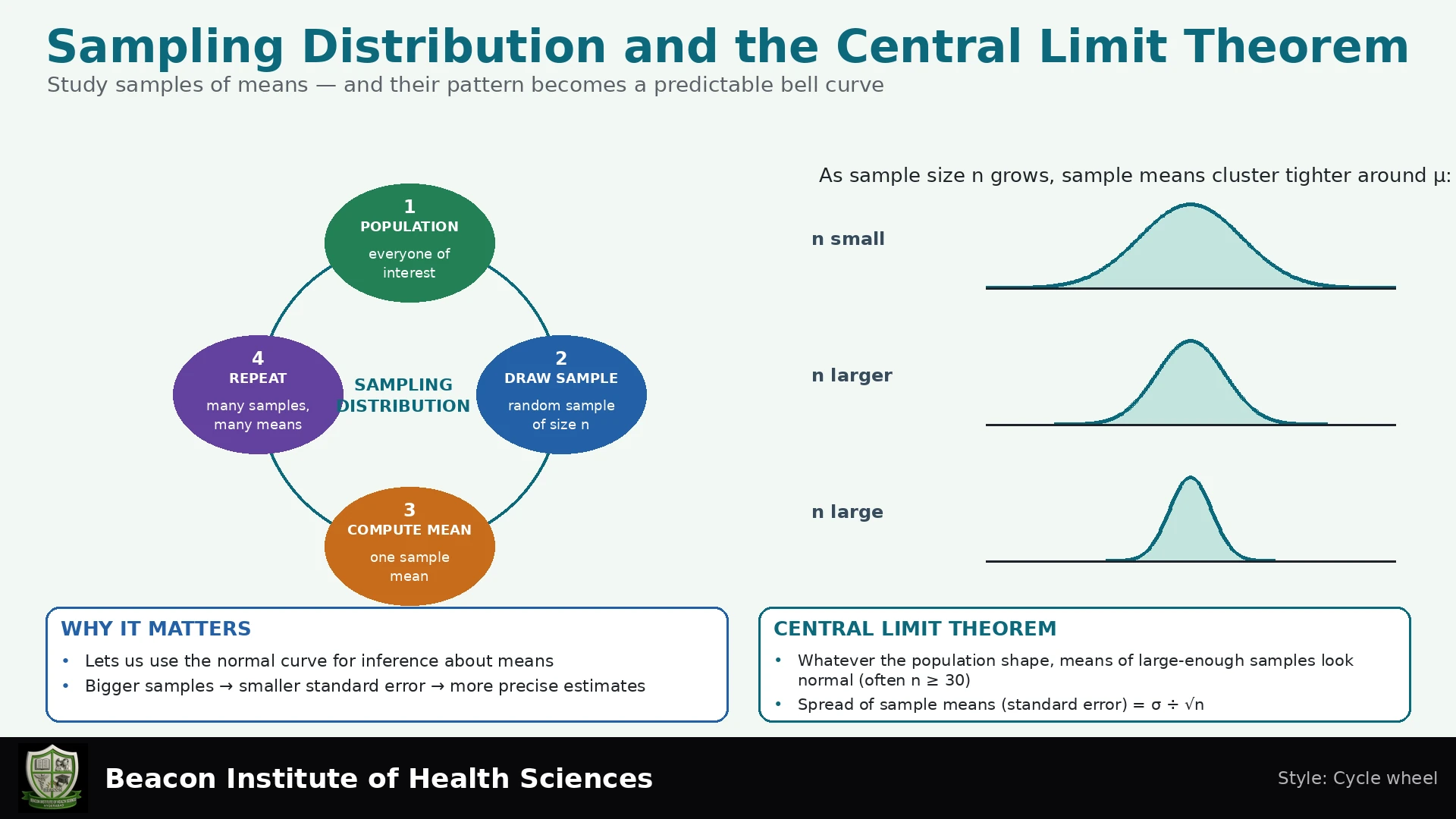
The sampling distribution of a statistic refers to the distribution of a specific statistic (e.g., the sample mean, x̄) calculated from repeated, same-size, independent random samples drawn from the same population. Imagine taking numerous samples of 100 adults, calculating the mean blood pressure for each sample, and then plotting all those sample means. The resulting distribution of these sample means is the sampling distribution of the mean.
Properties of the Sampling Distribution of the Mean
- Center: The mean of the sampling distribution of the mean (denoted μₓ̄) is equal to the population mean (μ). That is, μₓ̄ = μ.
- Spread (Standard Error): The standard deviation of the sampling distribution of the mean is called the Standard Error of the Mean (SE). It measures the variability of sample means around the true population mean.
- If the population standard deviation (σ) is known, and samples are independent and identically distributed (i.i.d.) with finite variance, the SE is calculated as:
SE = σ / √n - If the population standard deviation (σ) is unknown, the SE is estimated using the sample standard deviation (s):
Estimated SE = s / √n
- If the population standard deviation (σ) is known, and samples are independent and identically distributed (i.i.d.) with finite variance, the SE is calculated as:
Standard Deviation of Individual Observations vs. Standard Error of the Mean
| Characteristic | Standard Deviation (SD) | Standard Error (SE) |
|---|---|---|
| What it measures | Variability of individual data points within a single dataset (population or sample). | Variability of sample means (or other statistics) around the population parameter across multiple samples. |
| Formula (population) | σ | σ / √n |
| Interpretation | How much individual observations typically deviate from their mean. | How much sample means typically deviate from the population mean. |
| Relation to n | Population SD is a property of the population; estimated sample SD varies between samples. | Decreases as sample size (n) increases (specifically by a factor of √n). |
The Central Limit Theorem (CLT)
The Central Limit Theorem (CLT) is a fundamental theorem in statistics that has profound implications for nursing research. It states that, given a sufficiently large sample size, the sampling distribution of the sample mean will be approximately normally distributed, regardless of the shape of the original population distribution. This holds true provided the samples are independent and identically distributed (i.i.d.) and the population has a finite variance.
- Approximate Normality: As the sample size (n) grows, the standardized sample mean becomes approximately normally distributed.
- Exact Normality: If the population itself is already normally distributed, then the sampling distribution of the mean will be exactly normal for any sample size (n), assuming i.i.d. conditions.
- The 'n ≥ 30' Heuristic: Often, a sample size of 30 or more is considered a rule of thumb for the CLT to apply and for the sampling distribution to be approximately normal. However, this is a heuristic, not a guarantee. For populations that are highly skewed or have very heavy tails, a much larger sample size may be required for the sampling distribution to approximate normality.
What the CLT Does Not Do
- The CLT does not make the raw data from your observed sample normally distributed.
- It does not remove bias in sampling; a large biased sample will still yield biased results, regardless of the CLT.
- It does not fix issues of dependence or clustering within the data; if observations are not independent, simply increasing 'n' will not resolve this.
Finite Population Correction
When sampling a substantial fraction of a finite population (e.g., more than 5-10% of the population), a finite population correction factor may need to be applied to the standard error calculation to account for the reduced variability that occurs when a large portion of the population is sampled without replacement.
Illustrative Example: Applying the Concepts
Let's consider a synthetic population of patient satisfaction scores with a known mean (μ) of 40 and a standard deviation (σ) of 12. We want to understand the sampling distribution of the mean for different sample sizes.
Scenario 1: Sample Size (n) = 36
Using the formula SE = σ / √n:
SE = 12 / √36 = 12 / 6 = 2
Scenario 2: Sample Size (n) = 144
Using the formula SE = σ / √n:
SE = 12 / √144 = 12 / 12 = 1
Observation: Notice that when the sample size increases by a factor of four (from 36 to 144), the standard error is halved (from 2 to 1). This demonstrates how increasing sample size reduces the variability of sample means around the population mean.
Probability Calculation
If we assume the sampling distribution of the mean for n=36 is approximately normal due to the CLT, what is the probability that a random sample of 36 patients will have a mean satisfaction score above 44?
First, calculate the Z-score:
Z = (Sample Mean - Population Mean) / SE
Z = (44 - 40) / 2 = 4 / 2 = 2
Using a standard normal distribution table or calculator, the probability of Z > 2 is approximately 0.0228.
Important Note: This probability (0.0228) is for the sample mean being above 44. The probability for an individual depends on the population distribution and cannot be derived from the CLT for sample means alone. Individual SD is 12, not SE = 2. The sampling distribution is much narrower than the population distribution.
Clinical Relevance and Nursing Considerations
For BSN students and nursing educators, understanding sampling distributions and the CLT is vital for critically appraising research. Nurses routinely encounter research studies that use samples to make inferences about populations. A solid grasp of these concepts allows for a more informed evaluation of study validity, precision of estimates, and generalizability of findings.
- When reading nursing research, pay close attention to the sample design consistency. Inconsistent sampling methods can compromise the ability to generalize findings.
- Remember that large biased samples are not representative. The CLT does not correct for sampling bias; a large sample size alone does not ensure representativeness or validity if the sampling method itself is flawed.
Practice Questions & Solutions
Practice Question
In a second fictional teaching model, assume independent observations and an approximately normal sampling distribution of the mean. A population has an average score (μ) of 15 with a standard deviation (σ) of 4. A nurse researcher takes a random sample of 64 patients. What is the standard error of the mean for this sample, and what is the probability that the average score for this sample is less than 14?
Solution
1. Identify Given Information:
- Population Mean (μ) = 15
- Population Standard Deviation (σ) = 4
- Sample Size (n) = 64
- Desired Sample Mean (x̄) = 14
2. Calculate the Standard Error of the Mean (SE):
SE = σ / √n = 4 / √64 = 4 / 8 = 0.5
3. Calculate the Z-score for the Desired Sample Mean:
Z = (x̄ - μ) / SE = (14 - 15) / 0.5 = -1 / 0.5 = -2
4. Find the Probability:
We need to find P(X̄ < 14), which is equivalent to P(Z < -2). Using a standard normal distribution table or calculator, the probability for Z < -2 is approximately 0.0228.
Answer: The standard error of the mean for a sample of 64 patients is 0.5. The probability that the average score for this sample is less than 14 is approximately 0.0228.
Test your knowledge with our quiz:
https://bi.edu.pk/quiz-test/?quiz=sampling-distribution-and-the-central-limit-theorem
Review Questions
- What is plotted in a sampling distribution? A statistic from each possible or repeated same-size sample, such as one mean per sample. It does not plot individual patients from one sample.
- Does n = 30 guarantee a useful normal approximation? No. Skewness, heavy tails, dependence and the statistic being studied all matter.
- Will four times as many observations halve individual variability? No. Under the stated independent-sampling model, it halves the SE of the mean, not the population SD.
The numerical scores in both examples are invented for statistical learning. They do not represent a validated clinical risk scale or a patient-care cutoff.