
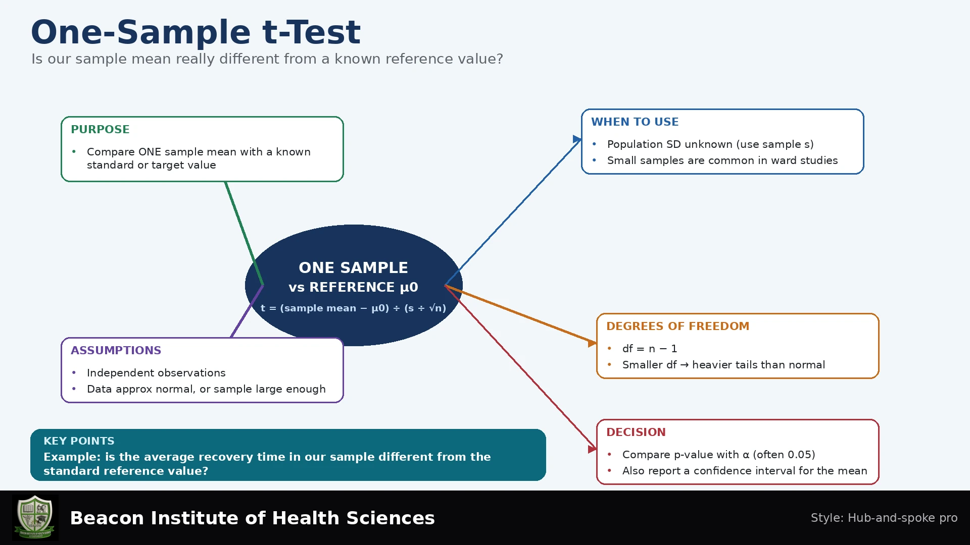
Introduction to the One-Sample t-Test
As BSN students and future healthcare professionals, understanding statistical methods is crucial for evidence-based practice. The one-sample t-test is a fundamental statistical tool used to compare the mean of a single numerical population to a known, fixed benchmark or hypothesized value when the population standard deviation is unknown. This lecture will guide you through its purpose, underlying assumptions, calculation, and interpretation, ensuring a solid foundation for its application in nursing research and clinical decision-making.
Learning Objectives
Upon completing this lesson, BSN students and educators will be able to:
- Define the purpose of the one-sample t-test.
- Formulate null and alternative hypotheses for a one-sample t-test.
- Identify and evaluate the key assumptions required for this test.
- Calculate the t-statistic and degrees of freedom for a given dataset.
- Interpret the results, including p-values and confidence intervals, in a nursing context.
- Distinguish between statistical and clinical significance.
- Understand how to report findings from a one-sample t-test.
What is the One-Sample t-Test?
The one-sample t-test is employed to determine if the mean of a sample (x̄) is significantly different from a pre-specified population mean (μ₀), often referred to as a benchmark or a target value, under circumstances where the population's standard deviation (σ) is unknown. For instance, a nurse researcher might use this test to compare the average pain score of a group of patients receiving a new intervention against a known standard pain score for a similar patient population.
Hypotheses
The test begins with formulating two opposing hypotheses:
- Null Hypothesis (H₀): The population mean (μ) is equal to the benchmark (μ₀). Statistically, this is written as H₀: μ = μ₀.
- Alternative Hypothesis (H₁): The population mean (μ) is not equal to the benchmark (μ₀). This can be a two-sided hypothesis (H₁: μ ≠ μ₀), or a one-sided hypothesis if a specific direction of difference is hypothesized beforehand (e.g., H₁: μ > μ₀ or H₁: μ < μ₀). The choice of one-sided or two-sided must be preset before data analysis.
Assumptions of the One-Sample t-Test
For the results of a one-sample t-test to be valid, certain assumptions about the data must be met:
- Independent Observations: Each observation in the sample must be independent of every other observation.
- Representativeness: The sample should be randomly selected and representative of the population from which it was drawn.
- Approximate Population Normality: The population from which the sample is drawn should be approximately normally distributed.
- Sample Size Considerations:
- For small sample sizes (small n), the normality assumption is more critical.
- For larger sample sizes (large n), the Central Limit Theorem suggests that the distribution of sample means will be approximately normal regardless of the population distribution, reducing the strict necessity for population normality. However, even with a large n, the presence of extreme outliers should still be carefully considered and does not automatically make the test robust against them.
- Data Type: The dependent variable (the data being measured) must be numerical and continuous. It is important to note that an ordinal single rating scale is not automatically considered a continuous variable for this test.
- Assumption Checks: Before conducting the test, it is crucial to check for these assumptions. Tools like histograms and QQ plots can help visualize the distribution and identify outliers. Outliers should not be automatically deleted; their presence requires careful consideration of their impact on the analysis.
Key Statistical Concepts
Standard Deviation (SD) vs. Standard Error (SE)
- Standard Deviation (SD): This describes the average amount of variability or dispersion of individual data points around the mean within a specific sample or population. It reflects the spread of data.
- Standard Error of the Mean (SE): This measures the accuracy with which a sample mean represents a population mean. It is the standard deviation of the sampling distribution of the mean, indicating how much sample means are expected to vary from the true population mean across different samples. The formula for the standard error of the mean is:
SE = s / √n
Where s is the sample standard deviation and n is the sample size.
Formulas for the One-Sample t-Test
The t-statistic quantifies the difference between the sample mean and the benchmark in terms of standard error units:
t = (x̄ - μ₀) / SE
Which can also be written as:
t = (x̄ - μ₀) / (s / √n)
Where:
x̄= sample meanμ₀= benchmark or hypothesized population means= sample standard deviationn= sample size
Degrees of Freedom (df)
The degrees of freedom for a one-sample t-test are calculated as:
df = n - 1
Confidence Interval (CI)
A 95% confidence interval is produced by a method that covers the fixed population mean in 95% of repeated samples under its assumptions. It does not assign a 95% probability to this particular interval. For the one-sample t-test, the confidence interval for the population mean is calculated as:
CI = x̄ ± tcritical * SE
Where tcritical is the critical t-value obtained from a t-distribution table based on the chosen alpha level and degrees of freedom.
Worked Example: Interpreting a One-Sample t-Test
Consider a synthetic dataset created for a nursing education scenario, where the goal is to compare a sample mean to a fixed benchmark. Imagine a group of 25 nursing students took a specialized assessment, and we want to compare their average score to a fictional fixed benchmark score of 50.
- Sample Size (n): 25
- Sample Mean (x̄): 52
- Sample Standard Deviation (s): 10
- Benchmark (μ₀): 50
Calculations:
- Calculate the Standard Error (SE):
SE = s / √n = 10 / √25 = 10 / 5 = 2 - Calculate the t-statistic:
t = (x̄ - μ₀) / SE = (52 - 50) / 2 = 2 / 2 = 1 - Determine Degrees of Freedom (df):
df = n - 1 = 25 - 1 = 24
Results and Interpretation:
For a two-sided test with df = 24 and the calculated t = 1, the approximate p-value is 0.327.
- 95% Confidence Interval (CI) for the mean: 47.87 to 56.13
- Difference between sample mean and benchmark: 2 (52 - 50)
- 95% CI for the difference: -2.13 to 6.13
Interpretation:
- Since the p-value (0.327) is greater than the conventional alpha level of 0.05, we fail to reject the null hypothesis. This suggests there is insufficient statistical evidence to conclude that the average score of this group of nursing students is significantly different from the benchmark of 50.
- The 95% Confidence Interval for the mean (47.87 to 56.13) includes the benchmark value of 50. This reinforces the conclusion that the sample mean is not significantly different from 50.
- The 95% Confidence Interval for the difference (-2.13 to 6.13) also includes zero, further supporting the failure to reject the null hypothesis.
It is crucial to remember that this example uses synthetic data and is for educational purposes only. No actual clinical findings are derived from this interpretation.
Important Considerations for Nurses
When interpreting the results of a one-sample t-test, BSN students must understand that failing to reject the null hypothesis does not mean that the null hypothesis is proven true. It simply means that there is not enough statistical evidence, based on the current sample, to conclude a difference exists. Furthermore, it is essential to distinguish between statistical significance and clinical significance. A statistically significant difference, especially with very large sample sizes, might not always represent a clinically meaningful effect. Always consider the effect difference in original units to gauge practical importance, not just the p-value.
Comparison of t-Tests
Understanding when to use different types of t-tests is vital:
| Test Type | Purpose | Comparison Scenario |
|---|---|---|
| One-Sample t-Test | Compares one numerical population mean with a fixed benchmark. | Is the mean blood pressure of a patient group different from a standard clinical guideline? |
| Independent Samples t-Test | Compares the means of two independent groups. | Is the mean pain score different between patients receiving intervention A versus intervention B? (Requires 2 sample comparison for an estimated benchmark, not a fixed one) |
| Paired Samples t-Test | Compares the means of two related groups. | Compare the mean within-student score change before and after teaching; analyze the paired differences. |
Reporting Results
When reporting the findings of a one-sample t-test, it is important to include comprehensive information for transparency and clarity. This typically includes:
- The sample mean (x̄)
- The sample standard deviation (s)
- The sample size (n)
- The calculated t-value
- The degrees of freedom (df)
- The p-value
- The Confidence Interval (CI) for the mean
Practice Questions
Why use t rather than z? The population standard deviation is unknown and is estimated using s. Does p = 0.327 prove equivalence? No; failing to reject a difference does not establish equivalence. What if the benchmark is an estimated mean from another sample? Its uncertainty must be considered, often through an independent two-sample analysis.
A two-sided p-value is the probability, assuming H₀ and the statistical model, of a t statistic at least as extreme in either direction as observed. It is not the probability that H₀ is true. Large samples do not repair dependent observations, biased selection, or all heavy-tailed distributions.
To further solidify your understanding of the one-sample t-test, please visit our interactive quiz:
Beacon Institute Quiz: One-Sample t-Test
Conclusion
The one-sample t-test is an invaluable statistical tool for BSN students and nursing professionals to compare a sample mean against a known standard or benchmark. By diligently applying its principles, understanding its assumptions, and correctly interpreting its results, nurses can contribute to evidence-based practice and make informed clinical judgments. Always remember to consider both statistical and clinical significance in your assessments.