
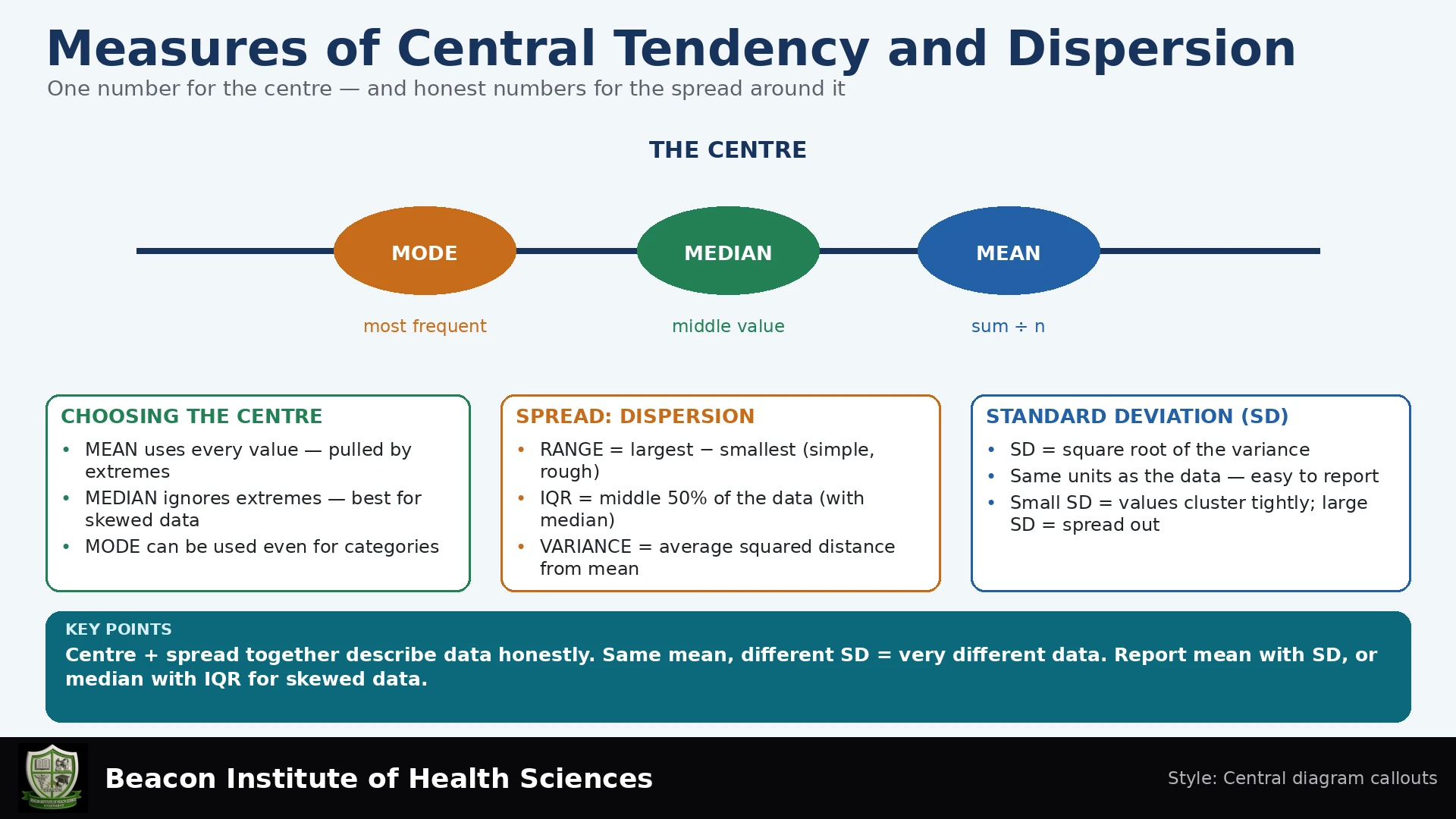
Understanding Central Tendency in Nursing Data
Measures of central tendency provide a single value that attempts to describe a set of data by identifying the central position within that data set. For nursing students, understanding these measures is crucial for interpreting research and patient data accurately.
Mean: The Arithmetic Average
The mean is the sum of all values divided by the number of values (n). It is calculated as:
Mean = Sum of all values / n
While commonly used, the mean is sensitive to outliers, meaning extreme values can significantly skew its representation of the data's center.
Median: The Middle Value
The median is the middle value in a dataset that has been ordered from lowest to highest. If there is an odd number of data points, the median is the single middle value. If there is an even number of data points, the median is the average of the two middle values. The median is robust to outliers, making it a valuable measure when extreme values are present.
Mode: The Most Frequent Value
The mode is the value that appears most frequently in a dataset. A dataset can have one mode, multiple modes, or no mode if all values appear with the same frequency. The mode is particularly useful for categorical data. It is important to note that using numerical codes for ordinal data does not justify calculating the mean for such data.
Comparison of Central Tendency Measures
| Measure | When to Use | Characteristics/Limitations |
|---|---|---|
| Mean | Symmetrical distributions, interval/ratio data without extreme outliers | Sensitive to outliers, represents arithmetic average |
| Median | Skewed distributions, ordinal data, interval/ratio data with outliers | Robust to outliers, represents the middle value |
| Mode | Nominal or categorical data, identifying most common category | Can have multiple modes or no mode, not always a unique center |
Understanding Measures of Dispersion (Variability)
Measures of dispersion describe the spread or variability of the data points around the central tendency. This helps BSN students understand how consistent or varied observations are within a dataset.
Range: The Simplest Measure
The range is the difference between the maximum and minimum values in a dataset. It provides a quick, but often limited, understanding of the total spread.
Range = Maximum value - Minimum value
Interquartile Range (IQR): Variability of the Middle 50%
The Interquartile Range (IQR) measures the spread of the middle 50% of the data. It is calculated as the difference between the third quartile (Q3) and the first quartile (Q1).
IQR = Q3 - Q1
To calculate quartiles for an odd number of data points, common conventions involve explicitly excluding the median when dividing the dataset into halves to find Q1 and Q3. Note that quartile calculations can differ slightly depending on the software used.
Variance: Average of Squared Deviations
Variance measures the average of the squared differences from the mean. It quantifies how much individual data points deviate from the mean. For a sample, the formula for variance is:
Sample Variance = Sum of (each value - mean)² / (n - 1)
Using (n-1) in the denominator for sample variance provides a better estimate of the population variance. For population variance, 'N' (total number of observations) is used as the denominator. Variance is expressed in squared units, which can make it less intuitive to interpret.
Standard Deviation (SD): Original Units of Variability
The standard deviation (SD) is the square root of the variance. It returns the measure of spread to the original units of the data, making it more interpretable than variance. For a sample, the formula for standard deviation is:
Sample SD = √Sample Variance
It's important to distinguish between standard deviation (SD) and standard error (SE), as they represent different concepts related to variability and sampling distributions.
Coefficient of Variation (CV): Relative Variability
The Coefficient of Variation (CV) is a measure of relative variability, expressed as a percentage. It is the ratio of the standard deviation to the mean. CV is only appropriate for data measured on a meaningful ratio scale with a non-zero positive mean (e.g., weight in kilograms), and it is not appropriate for scales like Celsius temperature, where zero is arbitrary.
Worked Teaching Example: Patient Wait Times
Let's consider an invented teaching example of patient wait times (in minutes) at a clinic: 2, 4, 4, 6, 9.
Initial Data Analysis (n=5)
- Sum: 2 + 4 + 4 + 6 + 9 = 25
- Mean: 25 / 5 = 5 minutes
- Ordered Data: 2, 4, 4, 6, 9
- Median: The middle value is 4 minutes.
- Mode: The most frequent value is 4 minutes.
- Range: 9 - 2 = 7 minutes
- Sum of Squared Deviations from the Mean:
(2-5)² + (4-5)² + (4-5)² + (6-5)² + (9-5)²
= (-3)² + (-1)² + (-1)² + (1)² + (4)²
= 9 + 1 + 1 + 1 + 16 = 28 - Sample Variance: 28 / (5 - 1) = 28 / 4 = 7
- Sample Standard Deviation: √7 ≈ 2.64575 (approximately 2.65 minutes)
- Quartiles (using median halves, excluding median):
Lower half: {2, 4}. Q1 = (2+4)/2 = 3 minutes.
Upper half: {6, 9}. Q3 = (6+9)/2 = 7.5 minutes.
Interquartile Range (IQR): 7.5 - 3 = 4.5 minutes
Impact of an Outlier
Now, let's observe the effect of an outlier by replacing the wait time of 9 minutes with an invented value of 29 minutes. New data: 2, 4, 4, 6, 29.
- New Sum: 2 + 4 + 4 + 6 + 29 = 45
- New Mean: 45 / 5 = 9 minutes (Notice the significant change from 5 to 9 minutes, demonstrating sensitivity to outliers).
- Ordered Data: 2, 4, 4, 6, 29
- Median: The middle value is still 4 minutes (The median remains robust to the outlier).
- Mode: The most frequent value is still 4 minutes (The mode happens to be unchanged in this example).
This example clearly illustrates how the mean is affected by extreme values, while the median and mode are unchanged in this particular dataset, highlighting their respective strengths and weaknesses.
Clinical Relevance and Safe Nursing Considerations
In nursing, these statistical measures help analyze data from patient populations, treatment effectiveness, and healthcare outcomes. It's crucial for BSN students to understand that these measures help interpret the distribution and characteristics of a sample or population. They should not be used as direct benchmarks for individual patient care without appropriate clinical context and further evidence-based guidelines.
Nursing Research Reading Checklist
A solid understanding of central tendency and dispersion is fundamental for critically appraising nursing research. When reviewing studies, nurses should assess how these measures are reported and interpreted, ensuring the chosen statistics are appropriate for the data type and study design.
Practice Answers Review
The worked example above provides detailed calculations for central tendency and dispersion for a given dataset, including the demonstration of outlier impact. Reviewing these steps reinforces the practical application of each formula and concept.
Understanding both central tendency and dispersion provides a comprehensive picture of any dataset, allowing BSN students and nursing educators to make more informed decisions based on data characteristics. This foundational statistical knowledge is indispensable for evidence-based practice and research in nursing.
You can test your knowledge with this quiz: https://bi.edu.pk/quiz-test/?quiz=measures-of-central-tendency-and-dispersion
Learning Objectives
- Calculate and interpret mean, median, mode and spread.
- Recognize the influence of extreme observations.
- Distinguish variability of individuals from precision of an estimated mean.
Explained Practice Questions
- What are the units of variance in this example? Minutes squared. The sample SD returns to minutes, which is why it is easier to interpret alongside mean waiting time.
- Does a median of four minutes mean everyone waited four minutes? No. It describes the central position of the ordered observations; the range and IQR reveal spread.
- Is SD the same as standard error? No. SD describes variation among observations. For independent, identically distributed observations, the estimated SE of the sample mean is s / √n. For this example it is √7 / √5 ≈ 1.18 minutes.
- Should the value 29 be removed automatically? No. Check for recording error, confirm the definition and investigate its context. A genuine unusual value may be important and should not be removed merely to improve a summary.
When reading a research table, check the variable's scale, units, denominator, missing entries, distribution shape, sample size and whether the reported “±” describes SD, SE or a confidence interval. These convey different information. Ask which quartile convention was used when reproducing an IQR.