
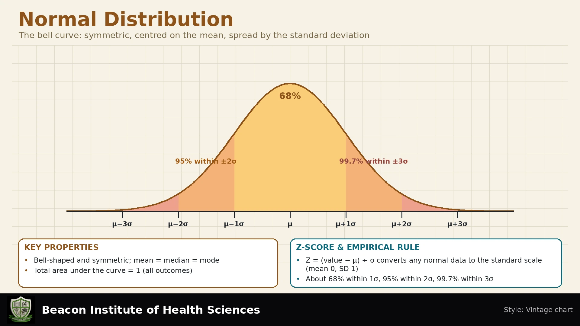
Introduction to Normal Distribution
The normal distribution is a fundamental concept in statistics, crucial for nursing students to understand as it underpins many statistical analyses encountered in healthcare research and evidence-based practice. This lesson will explore its characteristics, the standard normal distribution, and its application with a teaching example, alongside critical considerations for its use in health data.
Learning Objectives
Upon completion of this lesson, BSN students and nursing educators will be able to:
- Define the key characteristics of a normal distribution.
- Explain the concept of the standard normal distribution and Z-scores.
- Apply the empirical rule to interpret data within normal distributions.
- Calculate and interpret probabilities using a synthetic normal distribution example.
- Discuss the relevance and limitations of normal distribution assumptions in real-world health data.
Characteristics of the Normal Distribution
A normal distribution is a continuous probability distribution that is symmetric around its mean. It is often referred to as the "bell curve" due to its distinctive shape.
- Continuous: The variable can take any value within a given range.
- Symmetric Bell Shape: The distribution is perfectly symmetrical, meaning one side of the curve is a mirror image of the other.
- Mean, Median, and Mode are the Same: In a perfectly normal distribution, these three measures of central tendency all coincide at the peak of the curve.
- Total Area Under the Curve is 1 (or 100%): This represents the total probability of all possible outcomes.
- Tails are Unbounded (Theoretical): The tails of the curve extend infinitely in both directions, theoretically never touching the horizontal axis, though the probability beyond a few standard deviations becomes extremely small.
- Mean (μ): Defines the location or center of the distribution.
- Standard Deviation (σ): Determines the spread or dispersion of the distribution. A larger standard deviation indicates a wider, flatter curve, while a smaller standard deviation indicates a narrower, taller curve.
The Standard Normal Distribution and Z-Scores
The standard normal distribution is a special case of the normal distribution that is standardized. It has a mean (μ) of 0 and a standard deviation (σ) of 1. Any normal distribution can be converted to a standard normal distribution using a Z-score formula.
Z-Score Formula
The Z-score measures how many standard deviations an element is from the mean. It allows comparison of values from different normal distributions.
z = (x - μ) / σ
- x: The individual data point.
- μ: The population mean.
- σ: The population standard deviation.
- Dimensionless: Z-scores are dimensionless, meaning they do not have units.
- Probabilities and Areas: Z-scores are used to find probabilities, which correspond to the areas under the curve, not the height of the curve itself.
- Probability of a Single Exact Value: For a continuous distribution, the probability of a single exact value is theoretically 0. Probabilities are always calculated for intervals (e.g., between two values, above a value, or below a value), often involving rounding measured intervals.
The Empirical Rule (68-95-99.7 Rule)
This rule describes the approximate percentage of data points that fall within certain standard deviations from the mean in a normal distribution.
| Standard Deviations from Mean (±SD) | Approximate Percentage of Data |
|---|---|
| ±1 SD | 68.27% |
| ±2 SD | 95.45% |
| ±3 SD | 99.73% |
It is important to note that the central 95% of data falls within approximately ±1.96 standard deviations, not exactly ±2 standard deviations. This rule applies when the distribution is normal and is a statistical guideline, not a clinical rule for determining health or normalcy in individual patients.
Synthetic Teaching Example: Patient Waiting Times
Let's consider a synthetic model where patient waiting times in a clinic are normally distributed with a mean (μ) of 40 minutes and a standard deviation (σ) of 5 minutes. All numbers in this example are invented for teaching purposes and do not reflect actual clinical findings.
Problem 1: Probability of Waiting 50 Minutes or Less
What is the probability that a patient waits 50 minutes or less?
- Calculate the Z-score for x = 50 minutes:
z = (x - μ) / σz = (50 - 40) / 5 = 10 / 5 = 2 - Find the area corresponding to z = 2:
Using a standard normal distribution table or calculator, the area to the left of z = 2 (representing "50 minutes or less") is approximately 0.9772.
Therefore, there is a 97.72% probability that a patient waits 50 minutes or less.
- Calculate the right tail (waiting more than 50 minutes):
The area to the right of z = 2 is 1 - 0.9772 = 0.0228.
This means there is a 2.28% probability that a patient waits more than 50 minutes.
Problem 2: Probability of Waiting Between 30 and 50 Minutes
What is the probability that a patient waits between 30 minutes and 50 minutes?
- Calculate the Z-score for x = 30 minutes:
z = (30 - 40) / 5 = -10 / 5 = -2 - Recall the Z-score for x = 50 minutes:
z = 2(from Problem 1) - Find the area between z = -2 and z = 2:
According to the Empirical Rule, approximately 95.45% of data falls within ±2 standard deviations from the mean.
Alternatively, using a standard normal distribution table, the area to the left of z = 2 is 0.9772, and the area to the left of z = -2 is 0.0228.
The area between these two Z-scores is 0.9772 - 0.0228 = 0.9544.
Therefore, there is approximately a 95.44% probability that a patient waits between 30 and 50 minutes.
Model Suitability Note: In this theoretical model, negative waiting times are technically possible but have an infinitesimally tiny probability, but this fact alone does not establish model suitability. Actual waiting-time data must be assessed for skewness and other departures.
Clinical Relevance and Safe Nursing Considerations
While the normal distribution is a powerful statistical tool, its application in health data requires careful consideration.
- Real Health Data Variability: Real health data can often be skewed (e.g., length of hospital stay, cost of treatment), multimodal (having multiple peaks), or bounded (e.g., heart rate cannot be negative). It is critical not to assert that all health variables are normal.
- Checking for Normality: Nurses and researchers should always check the distribution of their data using graphical methods like histograms and Q-Q plots before assuming normality.
- Outliers: Outliers, extreme values in data, should not be deleted automatically. Their presence can significantly impact the mean and standard deviation and may indicate important clinical events or data errors.
- Normality for Statistical Models: Normality of raw observations or, more commonly, the residuals (errors) in a statistical model, is often an assumption for certain types of inferential statistics. Understanding this is crucial for interpreting research findings.
- Central Limit Theorem (CLT): The CLT states that the distribution of sample means (not raw observations) will tend to be normal, as sample size increases under suitable conditions, such as independent, identically distributed observations with finite variance. This is a crucial concept for hypothesis testing but does not mean individual patient data automatically becomes normal.
By understanding these nuances, BSN students can more accurately interpret statistical analyses in nursing research and apply evidence-based practice responsibly.
Test your knowledge with our quiz: Normal Distribution Quiz
Explained Practice Questions
- What is z for 35 minutes in this model? (35 − 40) / 5 = −1. The value is one standard deviation below the model mean.
- What interval contains the central 95%? 40 ± 1.96 × 5 gives approximately 30.2 to 49.8 minutes. This describes individual model values, not a confidence interval for an estimated population mean.
- Why do the two calculations give 95.44% and 95.45%? Subtracting rounded table entries gives 0.9544. Using more precise probabilities gives about 0.9545. The discrepancy is rounding, not a different distribution.
- Does being outside two SDs mean a patient is unwell? No. A statistical position under a model is not a clinical diagnosis or a treatment threshold.