
Introduction to Correlation
In nursing research and practice, understanding the relationships between different variables is crucial for informed decision-making and patient care. Correlation is a statistical measure that quantifies the extent to which two variables are linearly related. This lesson covers two primary types of correlation coefficients: Pearson's r and Spearman's rank correlation, exploring their properties, assumptions, calculation, and limitations.
Learning Objectives
Upon completing this lesson, BSN students and nursing educators will be able to:
- Define Pearson's r and Spearman's rank correlation coefficients.
- Interpret the sign, magnitude, and strength of correlation coefficients.
- Identify the key assumptions underlying Pearson's r for statistical inference.
- Perform a basic calculation of Pearson's r using synthetic data.
- Differentiate between correlation, causation, and agreement.
- Recognize common limitations and caveats in interpreting correlation analysis, such as the impact of outliers, range restriction, subgroups, and confounding.
- Understand appropriate reporting practices for correlation coefficients, including the importance of sample size (n), confidence intervals (CI), and uncertainty.
Understanding Pearson's r Correlation Coefficient
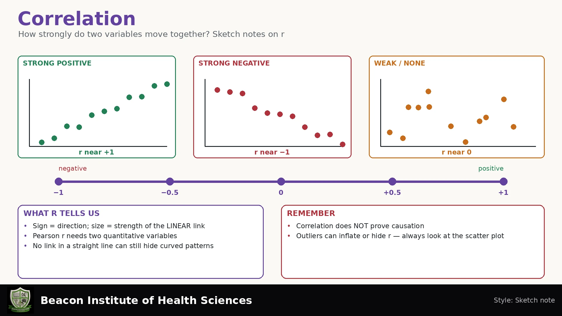
Pearson's r, also known as the Pearson product-moment correlation coefficient, is a widely used statistical measure. It is a unit-free, symmetric measure of linear association between two continuous variables. The value of Pearson's r ranges from -1 to +1.
- Sign and Direction: The sign of r (positive or negative) indicates the direction of the relationship. A positive r suggests that as one variable increases, the other also tends to increase. A negative r suggests that as one variable increases, the other tends to decrease.
- Magnitude and Strength: The absolute value of r indicates the strength of the linear relationship. A value closer to +1 or -1 indicates a stronger linear association, while a value closer to 0 indicates a weaker linear association.
- Nonlinear Relationships: It is important to note that a Pearson r value of zero indicates no linear relationship, but it may hide a strong nonlinear relationship between the variables. Therefore, visual inspection with a scatterplot is always recommended.
- Not Causation or Agreement: A crucial point for all correlation analyses is that correlation does not imply causation. Even a strong correlation between two variables does not mean that one variable causes the other. Similarly, correlation is not a measure of agreement between two variables.
Assumptions for Pearson's r (for Usual Inference)
While computing Pearson's r itself does not strictly require normal data, certain assumptions are typically made for usual statistical inference (e.g., hypothesis testing or constructing confidence intervals) about the population correlation coefficient:
- Independent Paired Observations: Each pair of observations (X, Y) must be independent of every other pair.
- Approximate Bivariate Normal Model: For standard inferential procedures, it is assumed that the data for the two variables (X and Y) are approximately bivariate normally distributed.
Worked Example: Calculating Pearson's r
Let's illustrate the calculation of Pearson's r using a synthetic dataset. This example will demonstrate the basic steps involved, highlighting the contributions of the sums of squares and cross-products.
Synthetic Data:
| X | Y |
|---|---|
| 1 | 2 |
| 2 | 4 |
| 3 | 5 |
| 4 | 4 |
| 5 | 5 |
Step 1: Calculate the Means of X and Y
- Mean of X (X̄) = (1 + 2 + 3 + 4 + 5) / 5 = 15 / 5 = 3
- Mean of Y (Ȳ) = (2 + 4 + 5 + 4 + 5) / 5 = 20 / 5 = 4
Step 2: Calculate the Sum of Squares and Cross-Products
These values are typically abbreviated as Sxx, Syy, and Sxy:
- Sxx (Sum of squares for X) = ∑(X - X̄)2 = (1-3)2 + (2-3)2 + (3-3)2 + (4-3)2 + (5-3)2 = (-2)2 + (-1)2 + (0)2 + (1)2 + (2)2 = 4 + 1 + 0 + 1 + 4 = 10
- Syy (Sum of squares for Y) = ∑(Y - Ȳ)2 = (2-4)2 + (4-4)2 + (5-4)2 + (4-4)2 + (5-4)2 = (-2)2 + (0)2 + (1)2 + (0)2 + (1)2 = 4 + 0 + 1 + 0 + 1 = 6
- Sxy (Sum of cross-products) = ∑((X - X̄)(Y - Ȳ)) = (-2)(-2) + (-1)(0) + (0)(1) + (1)(0) + (2)(1) = 4 + 0 + 0 + 0 + 2 = 6
The calculated sums are Sxx = 10, Syy = 6 and Sxy = 6.
Step 3: Calculate Pearson's r
The formula for Pearson's r is:
r = Sxy / sqrt(Sxx * Syy)
Plugging in our values:
r = 6 / sqrt(10 * 6)
r = 6 / sqrt(60)
r = 6 / 7.74596669
r ≈ 0.7745967
This calculated value of approximately 0.77 indicates a strong positive linear association between X and Y in this synthetic dataset.
Interpretation of r² (Coefficient of Determination)
The square of Pearson's r (r²) is also a significant statistic. In our example:
r² = (0.7745967)² ≈ 0.6
This value, r² = 0.6, represents the proportion of the sample Y variation that can be explained by simple linear regression with an intercept using X. It is critical to remember that r² does not imply causality, nor does it represent the percentage of patients or subjects explained by the relationship.
Understanding Spearman's Rank Correlation
Spearman's rank correlation coefficient (often denoted as ρ or rs) is another important measure of association. Unlike Pearson's r, which assesses linear relationships between continuous variables, Spearman's correlation is specifically designed for:
- Correlation of Ranks: It measures the monotonic relationship between two variables, meaning it assesses if the variables tend to move in the same direction, but not necessarily at a constant rate. This is achieved by ranking the data for each variable separately and then calculating Pearson's r on these ranks.
- Ordinal Variables: Spearman's correlation is particularly useful when dealing with ordinal variables (data that can be ranked but differences between values are not necessarily equal or meaningful) or when the assumption of bivariate normality for Pearson's r is violated.
- Handling Ties: When there are tied ranks in the data, it is important to average the ranks for these tied observations. Additionally, one should avoid using simplified formulas that assume no ties when ties are present, as this can lead to inaccurate results.
Limitations and Caveats in Correlation Analysis
While correlation is a powerful tool, its interpretation requires careful consideration of several factors:
- Not Causation or Agreement: As reiterated, correlation does not establish cause-and-effect or agreement. It only indicates a statistical association.
- Visual Inspection with Scatterplot: Always begin correlation analysis with a scatterplot. It can reveal nonlinear relationships that a Pearson r of zero might hide, and it helps identify other issues.
- Outliers: Extreme values, or outliers, can disproportionately influence the correlation coefficient, potentially inflating or deflating its value.
- Range Restriction: If the range of values for one or both variables is restricted in a sample, the calculated correlation may not accurately reflect the true correlation in the broader population.
- Subgroups: A correlation coefficient computed for an entire dataset might mask different or even opposite relationships existing within distinct subgroups of the data.
- Confounding: An observed correlation between two variables could be due to a third, unmeasured variable (a confounder) influencing both.
- Simpson's Paradox: This phenomenon occurs when a trend appears in several different groups of data but disappears or reverses when these groups are combined.
- No Universal Strength Cutoffs: Interpret strength in the scientific and measurement context; labels such as weak or strong have no universal numerical boundaries.
Reporting and Uncertainty
Distinguish sample r from the population correlation ρ that it estimates. State Pearson or Spearman, the number of complete pairs, coefficient, confidence interval, missing-data handling and scatterplot findings. A small sample can give a very uncertain estimate. A small p-value can occur for a weak correlation with a large sample and does not measure the strength or clinical importance of association.
A usual test of H₀: population Pearson correlation = 0 uses t = r√[(n − 2)/(1 − r²)] with n − 2 degrees of freedom under its model. Its p-value is the probability, assuming H₀ and the model, of a statistic at least as extreme as observed; it is not the probability that H₀ is true. Do not infer independence from a nonsignificant result.
Explained Practice
Can two devices correlate perfectly but disagree? Yes. If one device always reads 10 units higher, their readings can have r = 1 while showing systematic disagreement. Does r = 0 rule out association? No; a curved relationship can have little linear correlation. How should tied ordinal values be ranked for Spearman? Assign average ranks to ties and calculate correlation on those ranks using a method that handles ties.
In the fictional five-pair example, r ≈ 0.775 describes a positive linear sample association. It does not establish cause, an intervention benefit or reliable performance in new patients. Always interpret a correlation alongside its design, data quality and uncertainty.