
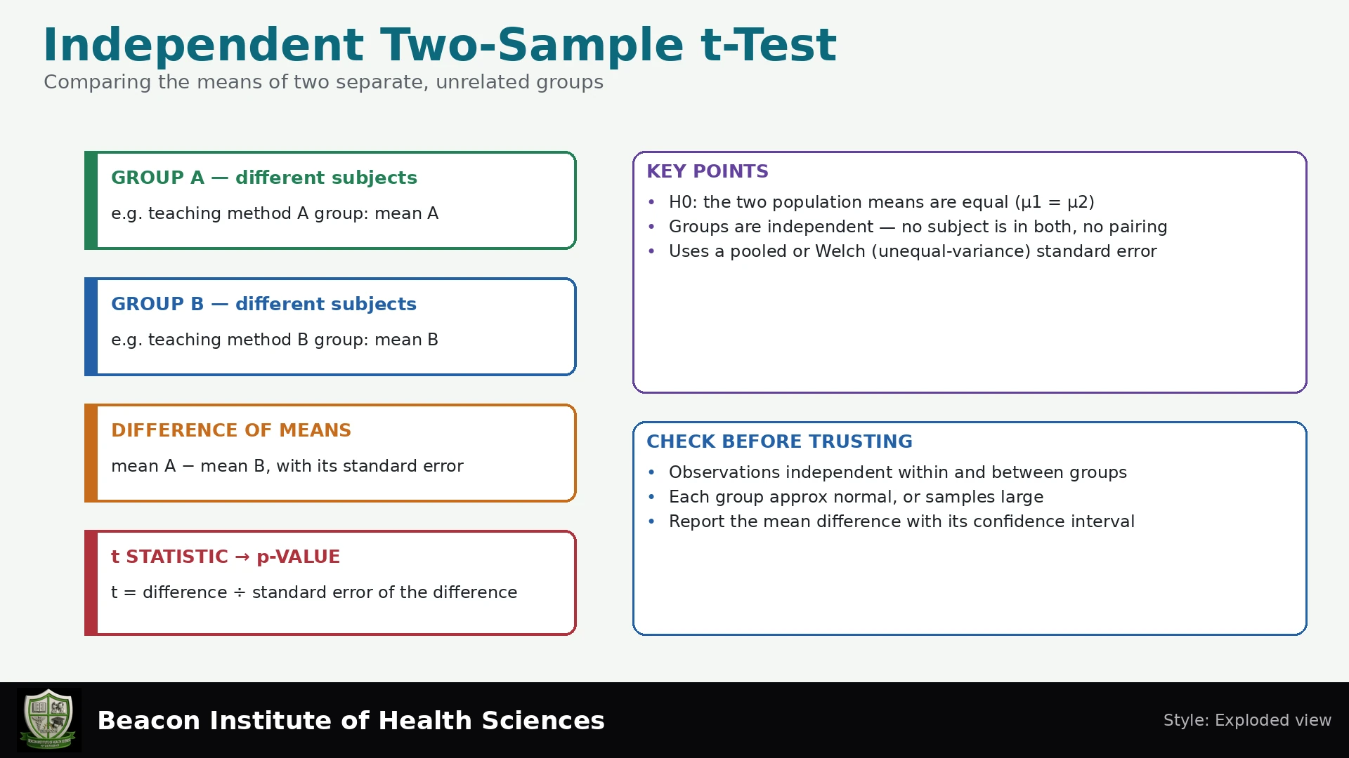
Introduction to the Independent Two-Sample t-Test
The independent two-sample t-test is a fundamental statistical tool in nursing research, used to compare the population means of two distinct, unrelated groups when the outcome variable is quantitative. This lecture will clarify its application, assumptions, and interpretation, equipping BSN students and educators with the knowledge to appropriately utilize and understand this test.
Learning Objectives
- Define the purpose and core characteristics of the independent two-sample t-test.
- Identify key assumptions required for valid application of the test.
- Distinguish between Welch's t-test and the pooled t-test.
- Understand the formulas for calculating the t-statistic and confidence intervals.
- Apply critical thinking to the clinical relevance and safe nursing considerations when interpreting t-test results.
- Work through a synthetic example to practice calculations and interpretation.
Understanding the Independent Two-Sample t-Test
The primary purpose of the independent two-sample t-test is to compare the population means of two independent groups with a quantitative outcome. This means the data for each group are collected from different participants, ensuring independence both within and between the groups.
Key Assumptions
For the independent two-sample t-test to provide valid inferences, several assumptions should be considered:
- Independence of Observations: The data points within each group, and between the groups, must be independent. This implies that the measurement for one participant does not influence or relate to the measurement of another. Instances like paired data (e.g., before-and-after measurements on the same person) or clustering (e.g., multiple patients from the same family or ward) violate this assumption, rendering the independent t-test inappropriate.
- Quantitative Outcome Variable: The variable being measured must be quantitative (interval or ratio scale).
- Normality within Groups: For small sample sizes (n) or in the absence of extreme outliers, the data within each group should be approximately normally distributed.
Welch's t-Test: A Robust Alternative
When conducting an independent two-sample t-test, a crucial consideration is whether the population variances of the two groups are equal. Welch's t-test does not assume equal population variance. This makes it a preferable general choice because it provides more robust results, especially when group sizes are unequal or variances are suspected to be different.
The Pooled t-Test: When Variances are Assumed Equal
In contrast, the pooled t-test assumes that the population variances of the two groups are equal. This assumption requires careful justification; one should not select solely based on a pretest for equal variances, as such pretests can be unreliable. If the equal variance assumption is met, the pooled t-test can be used, but Welch's test is often a safer default.
Formulas for the Independent Two-Sample t-Test
The calculation of the t-statistic and confidence interval are central to the independent two-sample t-test:
t-Statistic Formula (Welch's Test or general form)
The t-statistic is calculated as:
t = (x̄₁ - x̄₂ - δ₀) / √(s₁²/n₁ + s₂²/n₂)
x̄₁andx̄₂are the sample means of group 1 and group 2, respectively.s₁²ands₂²are the sample variances of group 1 and group 2, respectively.n₁andn₂are the sample sizes of group 1 and group 2, respectively.δ₀(delta zero) is the hypothesized difference between the population means (often 0 for a test of no difference).
Degrees of Freedom (df)
For Welch's t-test, the degrees of freedom are calculated using the complex Welch-Satterthwaite formula. It is important to note that the degrees of freedom are not automatically n₁ + n₂ - 2, which is typically used for the pooled t-test.
Confidence Interval (CI) for the Difference Between Means
The confidence interval for the difference between the two population means is calculated as:
CI = (x̄₁ - x̄₂) ± t_critical * SE
t_criticalis the critical t-value from the t-distribution corresponding to the chosen confidence level and degrees of freedom.SEis the standard error of the difference between the means, calculated as√(s₁²/n₁ + s₂²/n₂).
Clinical Relevance and Safe Nursing Considerations
Applying the independent two-sample t-test in nursing requires careful consideration of its implications:
- Observational vs. Causal: Remember that if your study design is observational, the test can indicate associations or differences, but it cannot establish causality.
- P-value Interpretation: A statistically significant p-value (e.g., p < 0.05) means that, under H₀ and the model, a t statistic at least as extreme as observed has probability below the chosen threshold. However, a p-value does not measure clinical benefit or practical importance. A statistically significant difference might not be clinically meaningful.
- Failing to Reject the Null: If you fail to reject the null hypothesis (i.e., p > 0.05), it means there isn't enough evidence to conclude a difference. However, failing to reject the null hypothesis is not evidence of equivalence.
- Units and Graphing: Always present estimates with appropriate units to give context. Visualizing data through graphs is highly recommended to understand distribution and potential outliers.
- Non-Parametric Alternatives: If the assumption of normality is severely violated, especially for small sample sizes, or if the data are ordinal, consider non-parametric alternatives such as the Wilcoxon rank-sum test. Note that the Wilcoxon rank-sum test compares ranks and distributions; a median-shift interpretation requires additional assumptions, which is not automatically the same as the mean.
- Synthetic Data for Learning: While worked examples use synthetic data for teaching purposes, remember that any synthetic teaching is not a clinical conclusion and should not be generalized to patient care.
Worked Example: Comparing Two Groups
Let's work through a synthetic example to apply the concepts learned. This is for teaching purposes only and does not represent a real clinical scenario.
Scenario and Given Data
A hypothetical study investigates the effectiveness of two different nursing interventions (Group 1 vs. Group 2) on a quantitative patient outcome score (e.g., pain level on a 0-20 scale). Data are collected from two independent groups.
- Group 1: Sample size (n₁) = 10, Sample mean (x̄₁) = 12, Sample standard deviation (s₁) = 3
- Group 2: Sample size (n₂) = 10, Sample mean (x̄₂) = 9, Sample standard deviation (s₂) = 3
Calculation Steps
- Calculate Sample Variances:
s₁² = 3² = 9
s₂² = 3² = 9 - Calculate the Standard Error (SE) of the Difference:
SE = √(s₁²/n₁ + s₂²/n₂) = √(9/10 + 9/10) = √(0.9 + 0.9) = √1.8 ≈ 1.34164 - Calculate the t-statistic (assuming δ₀ = 0 for no difference):
t = (x̄₁ - x̄₂ - 0) / SE = (12 - 9) / 1.34164 = 3 / 1.34164 ≈ 2.23607 - Determine Degrees of Freedom (df):
For these equal sample sizes and equal sample SDs, Welch’s formula also gives df = (0.9 + 0.9)² / [(0.9²/9) + (0.9²/9)] = 18. This coincides with the pooled-test df in this example; it is not the general Welch formula. - Find the p-value:
Using a t-distribution table or software with df = 18 and t = 2.23607, the two-tailed p-value is approximately 0.0382. - Calculate the 95% Confidence Interval for the Difference:
First, find the critical t-value for a 95% confidence level with df = 18. From tables, this is approximately 2.100922.
CI = (x̄₁ - x̄₂) ± t_critical * SE
CI = (12 - 9) ± 2.100922 * 1.34164
CI = 3 ± 2.81868
CI = (0.181 to 5.819)
Interpretation of Results
Based on our synthetic example:
- t-statistic (2.23607) and p-value (≈ 0.0382): Since the p-value (0.0382) is less than the common significance level of 0.05, we would reject the null hypothesis. This suggests a statistically significant difference in the mean outcome scores between Group 1 and Group 2.
- 95% Confidence Interval (0.181 to 5.819): This interval provides a range of plausible values for the true difference in population means. Since the entire interval (0.181 to 5.819) is above zero, it further supports the conclusion that the mean of Group 1 is significantly higher than Group 2. Specifically, we are 95% confident that the true difference in mean scores between Group 1 and Group 2 lies between 0.181 and 5.819.
Conclusion
The independent two-sample t-test is an indispensable tool for nurses and healthcare researchers to compare quantitative outcomes between two independent groups. Understanding its underlying assumptions, differentiating between Welch's and the pooled versions, and interpreting the results within a clinical context are vital skills. Always remember that statistical significance does not equate to clinical benefit, and caution is needed when drawing conclusions from observational studies.
You can test your understanding of the independent two-sample t-test with a short quiz:
Independent Two-Sample t-Test Quiz
Hypotheses and Worked Practice
For a two-sided comparison, H₀: μ₁ − μ₂ = 0 and H₁: μ₁ − μ₂ ≠ 0. Choose any one-sided alternative before examining results. Report the group means, SDs and sample sizes, the difference in original units, Welch t, fractional df where applicable, p-value and confidence interval.
Can repeated measurements on the same people use this test? No; use a paired or repeated-measures method. Does Welch remove the need to check independence? No. Why not automatically use df = n₁ + n₂ − 2? That is the pooled-test formula; Welch uses the sample variances and sample sizes in the Satterthwaite approximation.