Paired t-Test

Introduction to the Paired t-Test

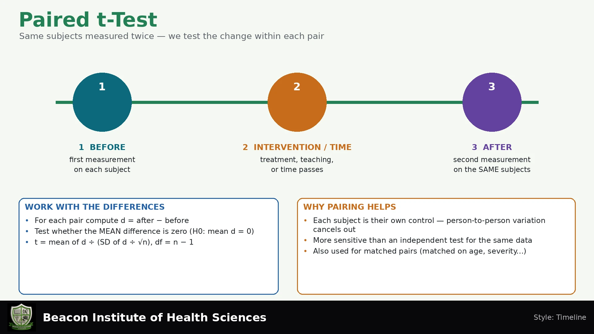
The paired t-test is a statistical hypothesis test used to compare the means of two related groups of samples. It is particularly valuable in nursing research for designs where measurements are taken on the same individuals under different conditions, or when natural pairing exists between subjects. This test focuses on the differences within each pair, making it suitable for 'before-after' studies or other matched-pair scenarios.

What is the Paired t-Test?

The paired t-test is designed to evaluate whether the mean of the differences between dependent observations is statistically significant. The core concept revolves around calculating the within-pair difference (d), typically defined as the 'after' measurement minus the 'before' measurement. While the pairs themselves are considered independent of one another, the observations within each pair are inherently dependent because they come from the same subject or a matched pair.

Assumptions of the Paired t-Test

For the paired t-test to provide valid results, certain assumptions about the data should be met:

• Dependent Samples: The data must consist of pairs of observations. These pairs could be measurements taken from the same individual at two different times (e.g., before and after an intervention) or measurements from two different individuals who have been matched based on relevant characteristics.
• Independence of Pairs: While observations within a pair are dependent, each pair must be independent of every other pair.
• Normality of Differences: The differences (d) between the paired observations should be approximately normally distributed. It is important to note that this assumption applies to the differences themselves, not necessarily to the raw 'before' and 'after' data points individually. For small sample sizes (n), inspection of the distribution of differences is crucial.
• Absence of Outliers: Outliers in the differences can unduly influence the test results. It is important to inspect the differences for any extreme values.

Formulating Hypotheses

In the context of the paired t-test, the hypotheses are stated in terms of the mean difference (μ_d) between the paired observations:

• Null Hypothesis (H₀): The true mean difference between the paired observations is zero. (H₀: μ_d = 0)
• Alternative Hypothesis (H_a): The true mean difference between the paired observations is not zero (for a two-sided test). (H_a: μ_d ≠ 0)

The Paired t-Test Formula

The test statistic for the paired t-test is calculated using the following formula:

t = d̄ / (s_d / √n)

Where:

• d̄ is the mean of the differences between the paired observations.
• s_d is the standard deviation of these differences, calculated as: s_d = √[Σ(d_i − d̄)² / (n − 1)]
• n is the number of complete pairs.
• √n is the square root of the number of pairs.

The degrees of freedom (df) for the paired t-test are calculated as:

df = number of complete pairs − 1

Confidence Interval for the Mean Difference

A confidence interval for the true mean difference (μ_d) provides a range of values within which the population mean difference is likely to fall. It is calculated as:

CI = d̄ ± t_critical × SE

Where:

• d̄ is the mean of the differences.
• t_critical is the critical t-value for a given alpha level (α) and degrees of freedom (df).
• SE is the standard error of the mean difference, calculated as: SE = s_d / √n

Important Considerations and Cautions

• Complete Pairs: Ensure that you only include complete pairs of data. Do not sort columns separately or impute missing values as zero, as this can severely bias your results.
• Direction of Difference: Reversing the direction of calculating differences (e.g., 'before' minus 'after' instead of 'after' minus 'before') will change the sign of the mean difference and the t-statistic, but it will not change the two-sided p-value.
• Causality in Pre/Post Designs: A pre/post design without a control group cannot establish causality. Observed changes might be due to regression to the mean, time-related practice effects, or other confounding factors, rather than solely the intervention itself.
• Paired vs. Two-Independent Samples: Understand the distinction between paired t-tests and two-independent samples t-tests. Using the wrong test can lead to incorrect conclusions.
• Attrition and Bias: In longitudinal studies, report any participant attrition and analyze potential biases that might arise from incomplete pairs.

Worked Example: Calculating the Paired t-Test

Let's consider a small, fictional sample of nursing students' scores on a knowledge assessment before and after an educational intervention. Assume appropriate distributions and no actual validated score or clinical data for this example.

Data:

Student	Before Score	After Score
1	10	11
2	12	14
3	11	14
4	13	17
5	14	19

Step 1: Calculate the Differences (d = After - Before)

• Student 1: 11 - 10 = 1
• Student 2: 14 - 12 = 2
• Student 3: 14 - 11 = 3
• Student 4: 17 - 13 = 4
• Student 5: 19 - 14 = 5

The differences are: 1, 2, 3, 4, 5.

Step 2: Determine the Number of Pairs (n)

There are 5 complete pairs, so n = 5.

Step 3: Calculate the Mean of the Differences (d̄)

d̄ = (1 + 2 + 3 + 4 + 5) / 5 = 3

Step 4: Calculate the Sum of Squares of Deviations (SSdev)

• (1 − 3)² = 4
• (2 − 3)² = 1
• (3 − 3)² = 0
• (4 − 3)² = 1
• (5 − 3)² = 4

SS = 4 + 1 + 0 + 1 + 4 = 10

Step 5: Calculate the Standard Deviation of the Differences (s_d)

s_d = √[10 / (5 − 1)] = √2.5 ≈ 1.58114

Step 6: Calculate the Standard Error of the Mean Difference (SE)

SE = 1.58114 / √5 ≈ 0.707107

Step 7: Calculate the t-statistic

t = 3 / 0.707107 ≈ 4.24264

Step 8: Determine Degrees of Freedom (df)

df = 5 − 1 = 4

Step 9: Determine the p-value and Confidence Interval

• For t = 4.24264 with df = 4, the two-sided p-value is approximately 0.01324.
• To calculate the 95% Confidence Interval, we use the critical t-value for df = 4 and α = 0.05 (two-tailed), which is approximately 2.776445.
• CI = 3 ± (2.776445 × 0.707107)
• CI = 3 ± 1.96324
• The 95% Confidence Interval is from 1.0368 to 4.9632.

Interpretation:

Given a p-value of 0.01324, which is less than the common significance level of 0.05, we would reject the null hypothesis. This indicates that there is a statistically significant mean difference in scores before and after the educational intervention. The confidence interval for the mean difference (1.0368 to 4.9632) does not include zero, further supporting the conclusion of a significant difference.

Alternative Non-Parametric Tests

If the assumption of normality for the differences is severely violated, especially with small sample sizes, or if the data are ordinal, non-parametric alternatives may be more appropriate. For paired data, the Wilcoxon Signed-Rank Test (which assesses symmetry of the distribution of differences) and the Sign Test (which focuses solely on the direction of differences) are two common non-parametric alternatives to consult.

Practice and Further Learning

Understanding the application and interpretation of the paired t-test is crucial for BSN students engaging in evidence-based practice and research. To further solidify your understanding, we encourage you to practice with various datasets and scenarios. An interactive quiz is available to test your knowledge: Paired t-Test Quiz.

Learning Objectives and Self-Check

After studying this lesson, identify paired designs, calculate within-pair changes, check assumptions, compute t and its confidence interval, and distinguish evidence of change from a causal effect.

Which distribution should be checked? The differences, especially with few pairs. Is n = 10 for five students measured twice? No; n = 5 complete pairs and df = 4. Does statistical significance show a useful intervention? No; interpret the estimated change and interval in original units and consider the study design.

The p-value assumes H₀ and the model and measures how unusual a statistic at least as extreme would be. It is not the probability that H₀ is true. A 95% confidence method covers the population mean change in 95% of repeated samples under its assumptions. Report complete-pair counts, mean change, SD of changes, t, df, p, interval, missingness and limitations.