
Regression in Biostatistics
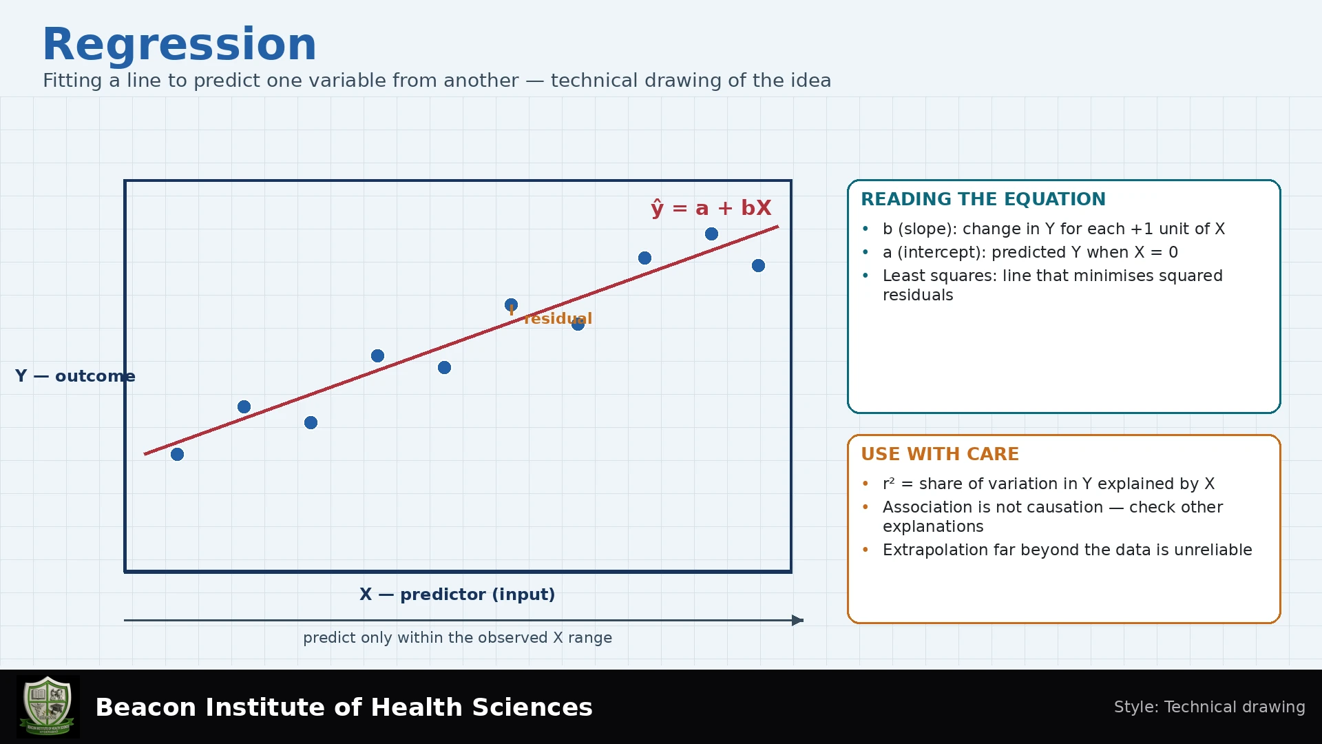
Regression describes how an outcome varies with one or more predictors. In nursing research it can help estimate associations, examine differences after adjustment, and develop predictions. The question and study design determine whether the fitted relationship is useful. An equation alone cannot establish that changing a predictor will change a patient's outcome.
Learning Objectives
- Identify the response, predictor, slope, intercept and residual.
- Calculate a simple least-squares line and interpret its units.
- Check assumptions and distinguish fitted values from reliable predictions.
- Explain uncertainty, R², extrapolation and limits of causal interpretation.
Model and Fitted Equation
For a quantitative outcome Y and numerical predictor X, the simple linear model is Y = β₀ + β₁X + ε. Its conditional mean is E(Y | X) = β₀ + β₁X: the average outcome at a specified predictor value. The error ε is the unobserved deviation from that population mean. A fitted sample equation is ŷ = b₀ + b₁x. A residual is the observed outcome minus its fitted value, e = y − ŷ. Errors and fitted residuals are related concepts, but are not identical.
The slope b₁ describes the estimated change in mean Y for a one-unit increase in X. Its units are outcome units per predictor unit. The intercept b₀ is the fitted mean when X is zero. If zero lies outside the observed range, the intercept may simply position the line and have little substantive meaning. A binary predictor can also be used in a linear model; it represents a group comparison. The simple numerical-predictor case is the focus here.
Least Squares
Least squares chooses the line that minimizes the sum of squared residuals. Let x̄ and ȳ denote sample means. Define Sxx = Σ(x − x̄)² and Sxy = Σ(x − x̄)(y − ȳ). Then b₁ = Sxy / Sxx and b₀ = ȳ − b₁x̄, provided X varies. The fitted line with an intercept passes through (x̄, ȳ). Squaring residuals makes large errors influential, so always inspect the scatterplot and unusual observations.
Worked Example Using Fictional Data
Five fictional students have study hours X = 1, 2, 3, 4, 5 and quiz points Y = 2, 4, 5, 4, 5. These small teaching data do not represent a clinical study or a validated educational scale.
| Hours x | Points y | Fitted ŷ | Residual y − ŷ |
|---|---|---|---|
| 1 | 2 | 2.8 | −0.8 |
| 2 | 4 | 3.4 | 0.6 |
| 3 | 5 | 4.0 | 1.0 |
| 4 | 4 | 4.6 | −0.6 |
| 5 | 5 | 5.2 | −0.2 |
The means are x̄ = 3 and ȳ = 4. Deviations of X are −2, −1, 0, 1, 2, giving Sxx = 10. Multiplying the paired X and Y deviations and summing gives Sxy = 6. Therefore b₁ = 6/10 = 0.6 points per study hour, and b₀ = 4 − 0.6 × 3 = 2.2 points. The equation is ŷ = 2.2 + 0.6x. At four hours it predicts 4.6 points; the observed four points give a residual of −0.6.
The residual sum of squares is SSE = 0.64 + 0.36 + 1 + 0.36 + 0.04 = 2.4. The total sum of squared Y deviations is SST = 6. Thus R² = 1 − SSE/SST = 1 − 2.4/6 = 0.60. In this sample, the fitted line explains 60% of variation in quiz points around their mean. This does not mean studying causes 60% of achievement, that 60% of students improve, or that predictions will have the same accuracy in a new population.
Assumptions and Diagnostics
- Linearity: the conditional mean follows the specified linear form. Curvature in residuals suggests a missing pattern.
- Independence: errors are independent under the design. Repeated measurements, wards and households may require models accounting for dependence.
- Constant error variance: the usual model assumes similar residual spread across fitted values. A funnel shape suggests unequal variance.
- Normal errors: approximate error normality supports usual small-sample t tests and confidence intervals. X itself does not need to be normally distributed.
Inspect residual-versus-fitted plots, a residual Q–Q plot, and influential observations. Investigate recording mistakes without deleting inconvenient points merely to improve significance. A small dataset cannot provide convincing diagnostic reassurance. Representative sampling, measurement quality and appropriate model specification remain necessary; a large sample does not correct systematic bias.
Inference and Prediction
A confidence interval for a slope describes uncertainty in the population association under model assumptions. A test of H₀: β₁ = 0 concerns the linear slope. Its p-value is calculated assuming H₀ and the model; it is not the probability that the null is true. Report the slope and interval in meaningful units, rather than significance alone.
A confidence interval for the mean response at a given X estimates the average outcome. A prediction interval for a new individual includes individual variation and is wider at the same X and confidence level. Predicting at six hours in this example is extrapolation beyond the observed one-to-five-hour range. The line need not remain valid there. Validate prediction models on new data and assess errors in the intended population.
Extensions and Nursing Interpretation
Multiple linear regression includes several predictors. An adjusted coefficient describes an association conditional on included variables; adjustment does not eliminate all confounding or prove causality. Binary outcomes often require logistic regression, which models log odds. Exponentiated logistic coefficients are odds ratios, not automatically risk ratios. Select the model for the outcome and design, with statistical support when necessary.
Reporting and Self-Check
Report sample size, outcome and predictor definitions, fitted coefficients with units and confidence intervals, R², diagnostic findings, missing-data handling, and design limitations. Separate prediction performance from causal claims.
What does slope 0.6 mean? The fitted mean score rises 0.6 points per additional study hour within the modeled range. Why is a residual negative? The observed outcome lies below the fitted value. Does R² = 0.60 prove cause? No; it describes sample fit and can reflect confounding or other noncausal patterns.