
Introduction to Chi-Square and Contingency Tables
The Chi-Square (χ2) test of independence is a fundamental statistical tool in nursing, used to analyze associations between two categorical variables. This lesson explores its application using contingency tables, crucial for BSN students in interpreting data and evaluating research.
Understanding Contingency Tables
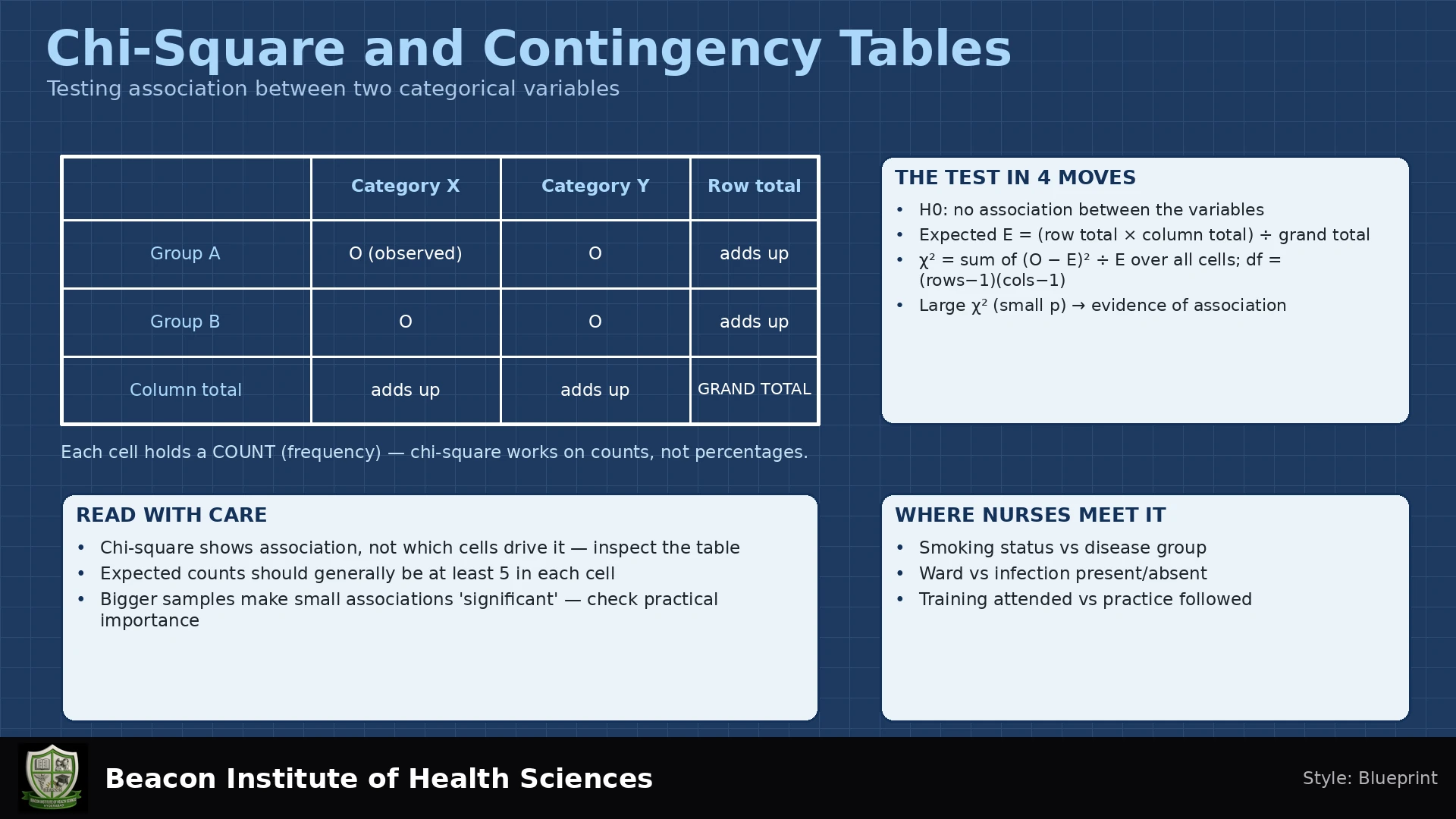
Contingency tables organize counts for two categorical variables into mutually exclusive cells. Each independent observation belongs to one cell. They feature rows, columns, and marginal totals (row totals, column totals), with N as the grand total. These totals serve as denominators for percentages and expected frequency calculations.
Hypothesis Testing with Chi-Square
The Chi-Square test evaluates if two variables are independent.
- Null Hypothesis (H₀): The variables are independent (no association).
- Alternative Hypothesis (H₁): The variables are associated (not independent).
The test compares observed frequencies to expected frequencies, which are the counts anticipated if H₀ were true.
Assumptions for the Chi-Square Test
Valid Chi-Square test results depend on key assumptions:
- Independent Observations: Each case is counted in only one cell ('one case one cell').
- Expected Frequencies: The test relies on expected, not observed, counts. A conservative criterion is 'all expected frequencies ≥ 5'. Rules vary; generally, 'none < 1' and 'most ≥ 5' is acceptable. Violation, especially in sparse 2 × 2 tables, may necessitate Fisher’s exact test or an appropriate exact or simulation-based method tests.
Calculating the Chi-Square Statistic
The Chi-Square statistic quantifies discrepancies between observed (O) and expected (E) frequencies.
Expected Frequency (E): E = (Row Total × Column Total) / N
Chi-Square (χ2) Statistic: χ2 = Σ((O - E)2 / E)
Degrees of Freedom (df): df = (Number of Rows - 1) × (Number of Columns - 1)
The Chi-Square test is a right-tailed test.
Worked Example: Interventions and Outcomes
Consider synthetic data on two fictional teaching groups (Group A, Group B) and assessment outcomes (Pass/Fail).
Observed Frequencies (O):
| Pass | Fail | Row Total | |
|---|---|---|---|
| Group A | 20 | 10 | 30 |
| Group B | 10 | 20 | 30 |
| Column Total | 30 | 30 | N = 60 |
Step 1: Calculate Expected Frequencies (E). N = 60.
For each cell, E = (30 × 30) / 60 = 15. .
All expected frequencies (15) are ≥ 5.
Step 2: Calculate (O - E)2 / E for each cell.
- (Group A, Pass): (20 - 15)2 / 15 = 25 / 15 = 1.6666667
- (Group A, Fail): (10 - 15)2 / 15 = 25 / 15 = 1.6666667
- (Group B, Pass): (10 - 15)2 / 15 = 25 / 15 = 1.6666667
- (Group B, Fail): (20 - 15)2 / 15 = 25 / 15 = 1.6666667
Step 3: Sum to get χ2.χ2 = 1.6666667 × 4 = 6.6666667 .
Specify no Yates continuity correction.
Step 4: Calculate Degrees of Freedom (df).df = (2 - 1) × (2 - 1) = 1 .
Step 5: P-value.
With χ2 = 6.6666667 and df = 1, p = 0.00982327.
Observed: Group A Pass 66.7% vs Group B Pass 33.3%.
Interpreting Results and Measures of Association
A p-value of 0.00982327 (< 0.05) indicates a statistically significant association between intervention and outcome. There is evidence against independence under the model. However, The statistic alone does not establish causality or specify the direction of association.
To quantify association strength:
- Phi Coefficient (φ) (for 2x2):
φ = √(χ2 / N)
φ = √(6.6666667 / 60) = √0.1111111 ≈ 0.333. - Cramer's V:
√(χ2 / (N × min(r-1, c-1))). For 2x2, it equals Phi.
Limitations of the Chi-Square Test
Key limitations include:
- Expected Frequencies: Violations require Fisher’s exact test or an appropriate exact or simulation-based method for sparse 2 × 2 tables.
- No Causation: χ2 shows association, not cause or direction.
- Non-Significant Result: Is not proof of independence.
- Paired Data: Use McNemar’s test for paired binary data.
- Clustering: requires analysis that accounts for the sampling design.
- Post-Hoc Analysis: cell-residual comparisons require a planned approach and multiplicity adjustment.
Reporting Chi-Square Results
When reporting Chi-Square results, ensure you include:
- Full observed/expected table.
- χ2 value.
- df.
- p-value.
- N.
- no Yates continuity correction (if applicable).
- Percentages (e.g., pass percentages of 66.7% and 33.3%).
- Measures of association (Phi/Cramer's V).
Self-Check Questions
Question 1
What determines the validity of the Chi-Square approximation?
Explanation: The validity of the Chi-Square approximation is determined by the expected counts, not the observed counts. Specifically, the assumption that all expected frequencies are ≥ 5 (or similar rules like 'none < 1, most ≥ 5') is critical.
Question 2
If a Chi-Square test yields a non-significant p-value, what can be concluded about the independence of the variables?
Explanation: A non-significant p-value means there is insufficient evidence to reject the null hypothesis of independence. However, it is not proof of independence; it merely indicates that the data do not provide strong enough evidence to claim an association.
Question 3
Which test is more appropriate for analyzing paired binary data, and why?
Explanation: For paired binary data, the McNemar’s test test is more appropriate than the Chi-Square test because it accounts for the dependency between observations (e.g., measurements taken from the same subject before and after an intervention), whereas Chi-Square assumes independent observations.
To further test your understanding, access the matching quiz here: Chi-Square and Contingency Tables Quiz
Conclusion
Chi-Square and contingency tables are vital for BSN students and nursing professionals, offering a structured approach to analyze categorical data. Mastering this statistical test enhances the ability to interpret research, evaluate interventions, and contribute to evidence-based healthcare practices.
Learning Objectives and Interpretation in Practice
After this lesson, construct a contingency table, distinguish observed from expected counts, calculate Pearson χ² and degrees of freedom, interpret association with appropriate limits, and identify situations needing another method.
The expected table for this example has 15 in every cell: A-pass 15, A-fail 15, B-pass 15 and B-fail 15. The expected counts are calculated under independence and can be non-integers in other datasets. Do not round them before calculating contributions. Observed counts are people or cases, rather than percentages, means or a list of measurements.
For the row percentages here, the denominator is each group total of 30: 20/30 = 66.7% and 10/30 = 33.3%. Column percentages answer a different question, using the outcome total instead. Label the denominator clearly. The chi-square value is unchanged if row labels are swapped, which illustrates why its magnitude alone does not tell the direction.
The reported calculation is Pearson’s uncorrected chi-square test, without Yates continuity correction. Software using a correction may return another p-value. Under H₀ and the model, the p-value is the probability of a chi-square statistic at least as large as observed. It is not the probability that H₀ is true. Neither this p-value nor the effect size demonstrates a causal teaching benefit. All counts in this example are fictional.
Choose categories before inspecting results, explain missing-data exclusions, and avoid merging categories only to obtain significance. For larger tables, a significant omnibus result does not identify the particular cells responsible; follow-up analyses require an appropriate multiplicity plan. Report observed counts with expected values, N, percentages, test version, χ², df, p-value and effect size, together with design limitations.