Analysis of Variance

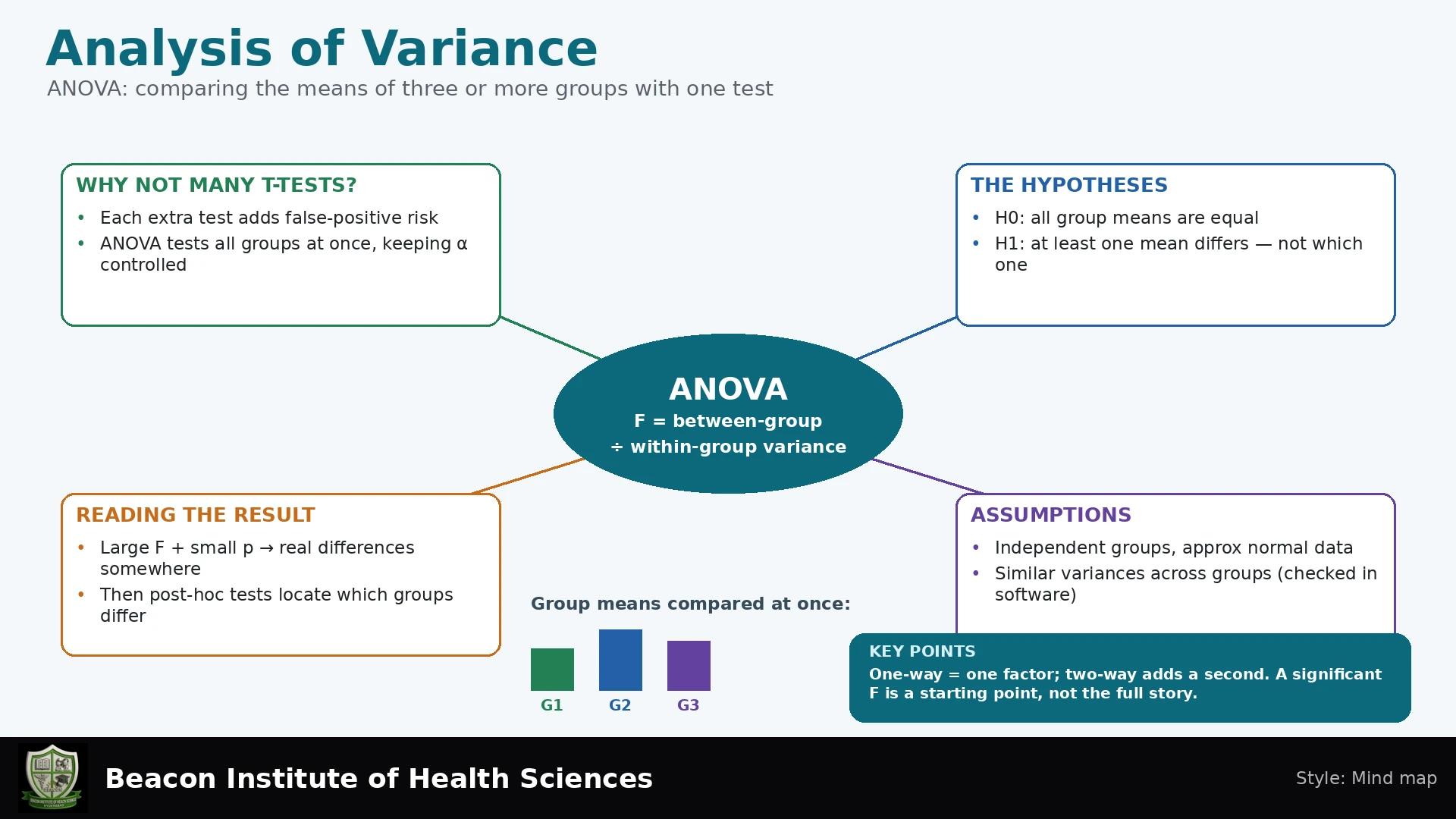
Introduction to Analysis of Variance (ANOVA)

As future healthcare professionals, Bachelor of Science in Nursing (BSN) students must develop a strong foundation in understanding statistical methods used in research and evidence-based practice. One such essential statistical tool is the Analysis of Variance, commonly known as ANOVA. This lesson introduces the One-Way Independent-Groups ANOVA, a method fundamental for comparing numerical outcomes across different groups.

By the end of this lesson, you will be able to:

• Understand the purpose and application of one-way independent-groups ANOVA.
• Formulate null and alternative hypotheses for ANOVA.
• Identify and explain the key components of ANOVA calculations, including Sums of Squares, Degrees of Freedom, and Mean Squares.
• Calculate and interpret the F-statistic.
• Recognize the critical assumptions underlying classical ANOVA.
• Discuss appropriate post-hoc tests and reporting standards.

What is One-Way Independent-Groups ANOVA?

One-way independent-groups ANOVA is a statistical test designed to compare a numerical outcome variable across several levels (or groups) of a single categorical independent factor. For instance, a nurse researcher might use it to compare the average pain scores (numerical outcome) among patients receiving different types of pain management interventions (categorical factor with multiple levels).

Formulating Hypotheses in ANOVA

Before conducting an ANOVA, we establish two competing hypotheses:

• Null Hypothesis (H₀): This hypothesis states that all population means across the different groups are the same. Symbolically, H₀: μ₁ = μ₂ = ... = μ_k, where μ represents the population mean for each of the K groups.
• Alternative Hypothesis (H₁): This hypothesis suggests that at least one population mean differs from the others. It is important to note that the alternative hypothesis does not claim that every pair of means is different, only that there is at least one significant difference among the group means.

Key Components of ANOVA Calculation

ANOVA works by partitioning the total variation observed in the data into different sources: variation between the groups and variation within the groups. These variations are quantified using Sums of Squares (SS).

Sums of Squares (SS)

• Sum of Squares Between Groups (SSB): This measures the variation between the means of the different groups. It reflects how much the group means deviate from the overall grand mean. The formula is: SSB = Σ n_j * (groupmean_j - grandmean)², where n_j is the number of observations in group j.
• Sum of Squares Within Groups (SSW): This measures the variation of individual observations within each group, around their respective group mean. It represents the random error or unexplained variance. The formula is: SSW = Σ (y_ij - groupmean_j)², where y_ij is the i-th observation in group j.
• Total Sum of Squares (TotalSS): This is the total variation in the entire dataset, representing the sum of the Sum of Squares Between Groups and the Sum of Squares Within Groups. TotalSS = SSB + SSW.

Degrees of Freedom (df)

Degrees of freedom are related to the number of independent pieces of information used to estimate a parameter. In ANOVA:

• Degrees of Freedom Between Groups (df_Between): K - 1, where K is the number of groups.
• Degrees of Freedom Within Groups (df_Within): N - K, where N is the total number of observations.
• Total Degrees of Freedom (df_Total): N - 1. Note that df_Total = df_Between + df_Within.

Mean Squares (MS)

Mean Squares are calculated by dividing the Sums of Squares by their respective degrees of freedom, providing an estimate of variance:

• Mean Square Between Groups (MSB): MSB = SSB / df_Between
• Mean Square Within Groups (MSW): MSW = SSW / df_Within

The F-Statistic

The F-statistic is the test statistic for ANOVA. It is a ratio of the variance between groups to the variance within groups:

F = MSB / MSW

A larger F-value indicates that the variation between group means is substantially greater than the variation within groups, suggesting that the group means are indeed different. Under H₀ and the classical assumptions, the statistic follows an F distribution with K − 1 numerator and N − K denominator degrees of freedom. The ANOVA rejection region is in the right tail.

Assumptions of Classical ANOVA

For the results of a classical ANOVA to be valid, certain assumptions about the data must be met:

• Independent Errors: Observations within and between groups must be independent of one another. This is typically ensured by random sampling and assignment in experimental designs.
• Approximately Normal Within-Group Errors: The residuals (the differences between observed values and group means) should be approximately normally distributed within each group. This assumption pertains to the population from which the samples are drawn.
• Equal Variances (Homoscedasticity): The variances of the outcome variable should be approximately equal across all groups.
• Not Pooled Normality: This refers to the assessment of normality, implying that normality is considered within each group rather than requiring the pooled raw outcome values to look normally distributed.

Diagnostic tools like residual plots can help assess these assumptions.

Addressing Assumption Violations

If assumptions are violated, alternative approaches may be necessary:

• Welch ANOVA: If the assumption of equal variances is violated, Welch ANOVA is a robust alternative that does not assume equal variances.
• Repeated Measures Methods: If data involve repeated measurements on the same subjects over time, specific repeated measures ANOVA methods are required, rather than independent-groups ANOVA.
• Non-parametric Tests: For severely non-normal data or when comparing medians, non-parametric tests like the Kruskal-Wallis test can be used. However, it's important to remember that Kruskal-Wallis is not a universal test of means; it compares rank distributions; a median-shift interpretation needs additional assumptions.

Worked Example: A Synthetic Data Scenario

Let's illustrate the ANOVA calculation with a synthetic dataset. Suppose we are comparing three different teaching methods (Group A, Group B, Group C) and measure student test scores (numerical outcome).

Synthetic Data

• Group A: Scores [2, 3, 4] → Mean_A = 3
• Group B: Scores [4, 5, 6] → Mean_B = 5
• Group C: Scores [6, 7, 8] → Mean_C = 7

From this data, we can determine:

• Total number of observations (N) = 9
• Grand Mean = (2+3+4+4+5+6+6+7+8) / 9 = 45 / 9 = 5
• Number of groups (K) = 3
• Number of observations per group (n_j) = 3 for each group.

Calculation of Sums of Squares

Sum of Squares Between Groups (SSB)

SSB = n_A*(Mean_A - Grand Mean)² + n_B*(Mean_B - Grand Mean)² + n_C*(Mean_C - Grand Mean)²

SSB = 3*(3 - 5)² + 3*(5 - 5)² + 3*(7 - 5)²

SSB = 3*(-2)² + 3*(0)² + 3*(2)²

SSB = 3*4 + 3*0 + 3*4

SSB = 12 + 0 + 12 = 24

Sum of Squares Within Groups (SSW)

SSW = Σ(y_ij - Mean_j)²

• For Group A: (2-3)² + (3-3)² + (4-3)² = (-1)² + 0² + 1² = 1 + 0 + 1 = 2
• For Group B: (4-5)² + (5-5)² + (6-5)² = (-1)² + 0² + 1² = 1 + 0 + 1 = 2
• For Group C: (6-7)² + (7-7)² + (8-7)² = (-1)² + 0² + 1² = 1 + 0 + 1 = 2

SSW = 2 (from A) + 2 (from B) + 2 (from C) = 6

Total Sum of Squares (TotalSS)

TotalSS = SSB + SSW = 24 + 6 = 30

Calculation of Degrees of Freedom

• df_Between = K - 1 = 3 - 1 = 2
• df_Within = N - K = 9 - 3 = 6
• df_Total = N - 1 = 9 - 1 = 8

Check: df_Total = df_Between + df_Within (8 = 2 + 6, which is correct).

Calculation of Mean Squares

• MSB = SSB / df_Between = 24 / 2 = 12
• MSW = SSW / df_Within = 6 / 6 = 1

Calculation of F-Statistic

F = MSB / MSW = 12 / 1 = 12

ANOVA Table Summary

The results are typically presented in an ANOVA table:

Source of Variation	Sum of Squares (SS)	Degrees of Freedom (df)	Mean Square (MS)	F	p-value
Between Groups	24	2	12	12	0.008
Within Groups	6	6	1
Total	30	8

Interpreting the Results

For our synthetic example, the calculated F-statistic is 12, with a p-value of 0.008. Given that a typical significance level (α) is 0.05, a p-value of 0.008 (which is less than 0.05) leads us to reject the null hypothesis (H₀). This indicates that there is a statistically significant difference among the means of the three teaching methods.

ANOVA is an omnibus test: rejection indicates at least one population mean differs under its assumptions. It does not identify which pair differs or show that every pair is different.

Post-Hoc Comparisons and Effect Size

If the scientific question requires pairwise follow-up, choose a justified method and account for multiple comparisons. Tukey comparisons are commonly used for all pairs in the equal-variance setting. Games–Howell comparisons can be considered with unequal variances. Planned contrasts should follow the prespecified research question. Running many unadjusted t-tests inflates the chance of false positive findings.

For the fictional example, η² = SSB / TotalSS = 24/30 = 0.80. This describes the fraction of sample variation associated with group membership in this fitted analysis. It does not establish a causal teaching effect or guarantee prediction performance in new students. With only three observations per group, assumptions are especially difficult to assess reliably.

Careful Interpretation and Reporting

For F(2, 6) = 12, the right-tail p-value is 0.008. Under the null hypothesis and model, it is the probability of an F statistic at least as large as observed. It is not the probability that H₀ is true or that the result is due to chance. Statistical significance does not establish educational or clinical importance. A nonsignificant ANOVA also does not prove that all means are equivalent.

Report group sample sizes, means and SDs, the ANOVA version, F with both degrees of freedom, p-value, effect size and uncertainty where appropriate, assumption checks, and any planned or post-hoc comparisons with their adjustment and confidence intervals. Describe missing-data handling, the sampling or allocation design and limitations. All scores above are synthetic teaching data, not actual study findings.

Explained Practice Questions

Why analyze variances when the question concerns means? The ratio compares variation between group means against variation within groups. Does significant ANOVA identify the best group? No; justified comparisons and the outcome direction are needed. Can ordinary independent-groups ANOVA analyze the same students at three times? No; dependence calls for a repeated-measures or other suitable model. What are the two degrees of freedom here? K − 1 = 2 and N − K = 6.